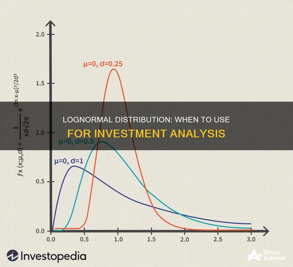
The lognormal distribution is a statistical concept used in financial modelling to determine the probability of an event occurring. It is particularly useful for modelling stock prices, as it assumes that stock prices cannot fall below zero and have an unlimited upside. This is in contrast to the normal distribution, which is symmetrical and allows for negative values. By using the lognormal distribution, investors can better identify the compound return that a stock can expect to achieve over time. This distribution is also used in the Black-Scholes option pricing model, which is a fundamental assumption in option pricing.
| Characteristics | Values |
|---|---|
| Shape | Right-skewed, with a long right tail |
| Mathematical Definition | If \(X\) follows a normal distribution with mean \(\mu\) and variance \(\sigma^2\), then \(Y = e^X\) follows a lognormal distribution |
| Positivity | Always positive |
| Multiplicative Nature | The product of lognormally distributed variables remains lognormally distributed |
| Extreme Values | More likely to occur than in a normal distribution |
| Application in Finance | Stock prices, option pricing, portfolio returns, and income modelling |
| Application in Other Fields | Particle sizes, species abundance, equipment reliability, project estimation, insurance claims, and credit risk |
What You'll Learn

Lognormal distribution for stock prices
The lognormal distribution is a common assumption used in stock price modelling. It is used to reflect the reality that stock prices cannot go negative and have unlimited upside potential. This is because the lognormal distribution is bound by zero on the lower side, making it suitable for modelling asset prices that cannot take negative values.
The lognormal distribution is used in stock price modelling because it aligns with the framework of stock prices, which are a function of the current price and the exponent of the expected return. This relationship is reflected in the lognormal distribution's framework, where the rate of return, if continuously compounded and normally distributed, results in the future stock price being modelled as lognormal.
To apply this concept, investors often transform daily holding period returns into continuously compounded returns. This involves using the natural logarithm to calculate the continuously compounded return, which is the log of the ending price over the beginning price. This practical approach allows investors to model stock price movements more accurately, considering the natural variability and growth potential inherent in financial markets.
The Black-Scholes model, used in pricing options, also uses the lognormal distribution as its foundation. This is because the lognormal distribution can capture the potential for large moves in cheap stocks, even if the price change is small. For example, a $0.10 reduction in a $2 stock is a 5% change. Therefore, while the stock return is normally distributed, the price movement is best explained using a lognormal distribution.
Robo-Advisers: Investment Advisers' Future or Fad?
You may want to see also

Lognormal distribution for option pricing
The lognormal distribution is a common assumption used in option pricing models, such as the Black-Scholes model. This model is widely used for pricing options and is based on the assumption that the underlying asset's price follows a lognormal distribution.
The lognormal distribution is a type of probability distribution that is positively skewed, meaning it has a long right tail and no negative values. This characteristic is important in financial modelling because it reflects the nature of stock prices, which cannot go negative and have the potential for unlimited upside.
By assuming that the underlying asset's price follows a lognormal distribution, the Black-Scholes model can be used to determine option prices. This is because the lognormal distribution of prices implies a normal distribution of returns, which can be modelled using the Black-Scholes equation.
The Black-Scholes-Merton model implies that the prices of the underlying asset at maturity ($S_T$) are log-normally distributed:
$ln(S_T)\sim N\big[ln(S_0)+(\mu-\frac{\sigma^2}{2})T,\;\sigma^2T\big]$
This equation states that the natural logarithm of the asset's price at maturity ($S_T$) is normally distributed, with a mean of $ln(S_0)+(\mu-\frac{\sigma^2}{2})T$ and a variance of $\sigma^2T$. Here, $S_0$ is the current price of the asset, $\mu$ is the expected return, $\sigma$ is the standard deviation of returns, and $T$ is the time to maturity.
By assuming lognormal distribution for option pricing, analysts can capture the inherent variability and growth potential in financial markets. This allows for more accurate modelling of stock price movements and, consequently, more informed investment decisions.
Understanding Investment Cash Flow Entries and Their Impact
You may want to see also

Lognormal distribution for portfolio returns
Lognormal distribution is a crucial concept in financial markets, especially when it comes to understanding portfolio returns and their impact on investment decisions.
When considering portfolio returns, it is essential to recognise the differences between lognormal and normal distributions. The normal distribution, often referred to as the bell curve distribution, is symmetrical, with 68% of results falling within one standard deviation and 95% within two standard deviations. On the other hand, the lognormal distribution is right-skewed, ensuring that values do not fall below zero. This skewness is a critical factor in determining which distribution to use when making investment choices.
The lognormal distribution is particularly useful when analysing stock prices. Since stocks grow at a compounded rate, the lognormal distribution can be applied when an investor wants to estimate a stock's future price. By using the current stock price and multiplying it by various rates of return, the investor can model the future stock price as lognormal. This approach is accurate because stock prices cannot go negative and have the potential for unlimited growth, aligning with the characteristics of the lognormal distribution.
However, when calculating total portfolio returns, the normal distribution is generally preferred. This is because the weighted average return, which considers the weight of each security in the portfolio, provides a more precise description of the actual portfolio return, taking into account both positive and negative returns. The lognormal distribution may be faster to calculate for long-term performance, but it fails to capture the individual stock weights, which can significantly impact the overall return.
Understanding the nuances between these distributions is essential for making informed decisions about portfolio returns and future stock prices. By grasping these concepts, investors can better navigate the complex world of financial investments and portfolio management.
Unlocking EPF for ASB Investment: A Guide
You may want to see also

Lognormal distribution for income modelling
Lognormal distribution is a common model used to study income inequality. It is defined by the mean wealth per capita as the central tendency and the Gini coefficient as a measure of dispersion. The lognormal distribution is skewed right, meaning it stretches out towards the right, creating a long tail. This characteristic ensures that values do not dip below zero.
The lognormal distribution is particularly useful for modelling stock prices because stock prices cannot fall below zero. To calculate expected stock prices, investors will take the current stock price and multiply it by various rates of return, which are mathematically derived exponential factors based on compounding. When the investor continuously compounds the returns, they create a lognormal distribution.
The lognormal distribution is also used in the Black-Scholes model for pricing options. However, the normal distribution is typically preferred when calculating total portfolio returns as it can capture both positive and negative returns.
The lognormal distribution is based on the assumption that the natural logarithm of a random variable (Y) is normally distributed. This means that if "the log is normal", then the variable is lognormally distributed. This assumption has practical applications in finance, particularly in accurately modelling stock price movements by taking into account natural variability and growth potential.
In terms of income modelling, the lognormal distribution has been studied and proposed as a tool for analysing the effects of anti-poverty policies. It has been found to adequately reproduce the lower tail and the kurtosis of income distribution. The lognormal distribution is also useful for modelling income data, especially in capturing the degree of kurtosis of empirical distributions.
Investing Wisely: Allocating Your Paycheck for Financial Freedom
You may want to see also

Lognormal distribution for credit risk
Lognormal distribution is a crucial concept in finance, and it has several applications in credit risk analysis. Credit risk distribution is the probability distribution of losses that a lender or investor may face due to a borrower's default or non-payment. This distribution is essential for measuring and managing credit risk exposure in a portfolio of loans, bonds, or other financial instruments.
The lognormal distribution is often used when credit risk exhibits positive skewness, meaning the tail of the distribution is skewed to the right. This distribution is particularly useful when modelling asset prices or credit losses. The key characteristic of the lognormal distribution is that it only produces positive values, making it suitable for modelling stock prices since they cannot fall below zero.
When analysing credit risk, the lognormal distribution is applied to model the potential losses incurred. The distribution is used to estimate the likelihood of extreme losses, with its right-skewed nature capturing the possibility of large losses. This is in contrast to the normal distribution, which assumes a stable and symmetric distribution of credit risk.
The choice between the lognormal and normal distributions depends on the specific characteristics of the credit portfolio and the objectives of the analysis. The lognormal distribution is preferred when dealing with asset prices or credit losses that can be highly variable and have an unlimited upside, such as stock prices.
Additionally, the lognormal distribution is used in the Black-Scholes model for options pricing. This model serves as the basis for determining option prices by incorporating the lognormal distribution to reflect the potential for gains and the inability for losses to extend beyond the initial investment amount.
In summary, the lognormal distribution is a valuable tool in credit risk analysis, especially when dealing with positive skewness, asset prices, and credit losses. It provides a more realistic representation of potential losses and is essential for effective risk management, pricing, and portfolio optimisation.
Maybank Investment Guide: Strategies for Smart Investing
You may want to see also
Frequently asked questions
The lognormal distribution is used when dealing with variables that exhibit multiplicative growth and are constrained to positive values. It is particularly useful when analyzing stock prices, as it reflects the reality that stock prices cannot go negative and have unlimited upside.
The lognormal distribution differs from the normal distribution in its shape. The normal distribution is symmetrical, forming a bell curve, while the lognormal distribution is right-skewed, meaning it stretches out to the right, creating a long tail. This is because the values in a lognormal distribution are positive.
The lognormal distribution can be calculated in Excel using the function LOGNORM.DIST (x, mean, standard_dev, cumulative). This function returns the lognormal distribution of x, where ln(x) is normally distributed with the specified mean and standard deviation.


